
Research commentary
Revisiting an old trading indicator is a little like returning to a restaurant you loved before you understood much about cooking. You still recognize what drew you in. You also start noticing how much you mistook presentation for proof.
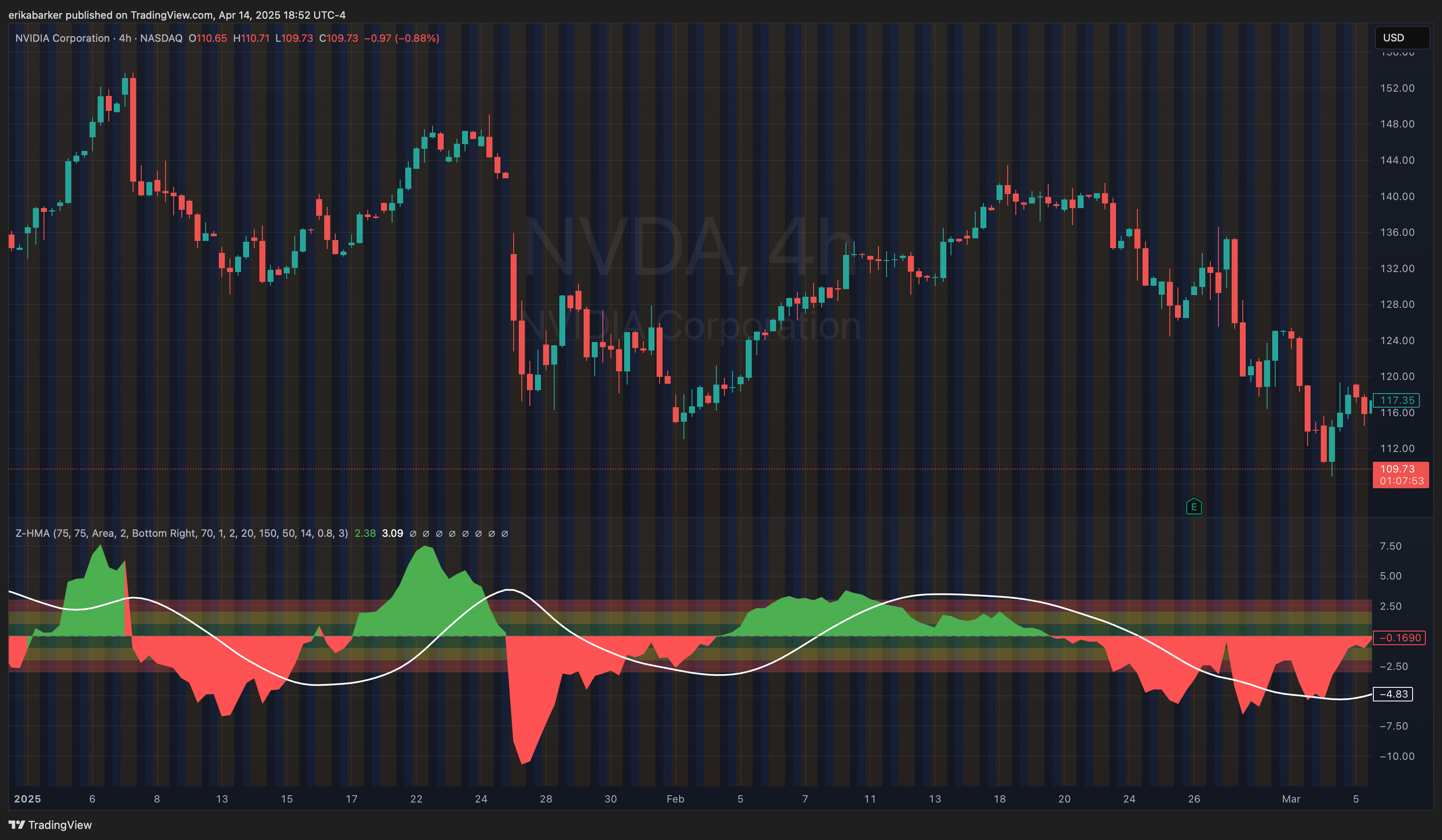
When I wrote about my HMA Z-score indicator in May 2024, I was excited about what a few mathematical ideas could reveal on a chart. I still am. But I read that article differently now, especially its language about probability and improved performance.
I now work at a quantitative research hedge fund. I have also made enough mistakes in my own research to become suspicious of the moment when the numbers start telling me exactly what I want to hear.
A smoother line can be useful. A higher backtest score can be interesting. Neither settles the question of whether a tool helps us understand a market, much less whether it will make money.
My latest Z-Score Probability Pro KAMA grew out of that distinction. It is the third published iteration of this KAMA project, and part of a longer journey that began with the HMA indicator. The most valuable changes reflect what I have learned about asking better questions.
What a Z-score can actually tell us
A Z-score expresses an observation’s distance from a mean in units of standard deviation. Standard deviation describes spread: how dispersed the observations are around their average.
Imagine a series with an average of 100 and a standard deviation of 5. An observation of 110 has a Z-score of +2. An observation of 90 has a Z-score of −2. That calculation describes the observation relative to the chosen reference.
It does not tell us that 90 is a bargain.
That was a distinction I needed to take more seriously. My earlier article connected extreme readings with possible reversals and described probability zones in language that could make a descriptive measurement sound like a forecast.
For a normal distribution, about 95.45% of observations fall within two standard deviations of the mean. That is a property of a specified distribution. It is not a 95.45% probability that a stock will reverse after touching a line. You can calculate a Z-score without assuming normality; translating it into normal-distribution odds requires assumptions that the calculation itself does not establish. NIST’s explanation makes the distributional meaning clear.
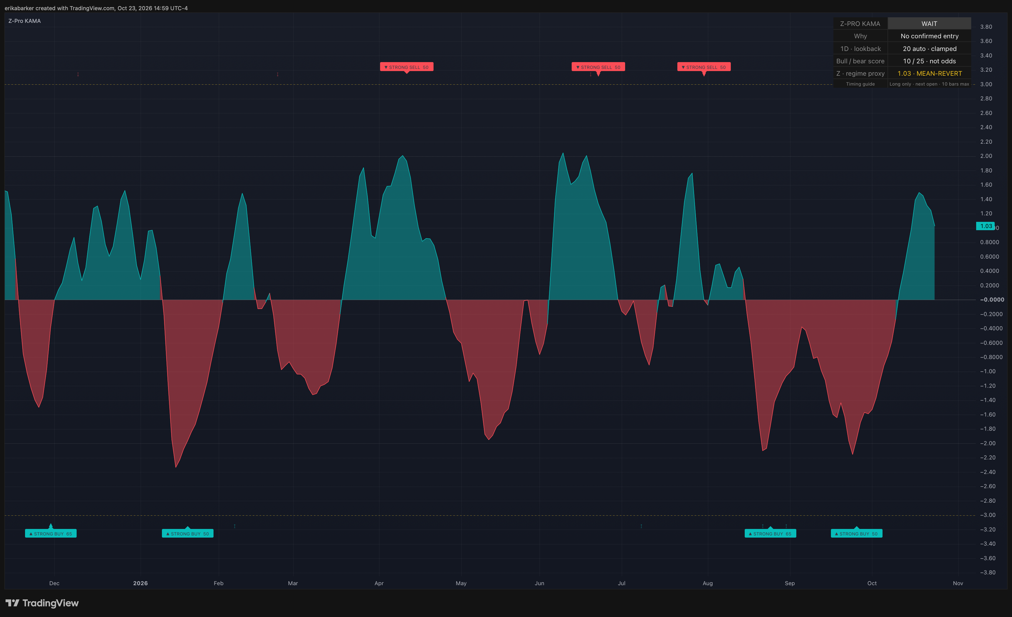
There is another wrinkle in the current indicator. Its default calculation standardizes the residual between price and an adaptive baseline, centering that residual around its own rolling mean. The displayed oscillator is then smoothed. A displayed −2 is therefore not simply “the stock is exactly two standard deviations below its raw price average.”
If we are going to use a number to guide a decision, we need to know which number we are looking at.
The temptation to keep improving the score
I went through a phase of leaning heavily on machine learning and parameter optimization. Change a lookback. Adjust a threshold. Try another combination. Keep the version that makes the results look better.
Optuna is an open-source framework for automating that search. You define the settings it can vary and an objective it should minimize or maximize. It runs trials and searches for settings that perform well against that objective. Those settings are often called hyperparameters: choices such as model depth, learning rate, or a signal’s lookback window.
Optuna does not decide whether your experiment answers the right question. If the objective rewards a flattering historical score, the search can become very good at producing one.
That is a problem with the research design, not a reason to declare optimization useless. It also exists when the optimizer is a human scrolling through charts and keeping the combinations they like.
The research on backtest overfitting by Bailey, Borwein, López de Prado and Zhu formalizes a familiar danger: selecting a strategy because it looks best in historical tests can produce an unreliable estimate of how it will perform elsewhere. Repeatedly inspecting and responding to results spends information, even when we continue calling part of the dataset a “test.”
My mental picture is a researcher who studies ten patients, keeps the ones who responded best, adjusts the intervention around them, and then expects the result to describe everyone. The problem is the selection and the leap to generalization. A carefully designed study of one person can answer a useful question about that person; it cannot automatically answer a population-level question.
A ticker can have a recognizable personality, but that personality is shorthand for things worth investigating: liquidity, investor participation, business exposure, volatility, and how it responds to information. It is not a permanent trait. Ten years of one instrument do not become ten independent markets because the spreadsheet has a lot of rows.
Two useful ingredients can make a worse model
I have also learned to be careful with combinations.
Two indicators can each be useful and still contribute very little together. If both are transformations of the same price history, their apparent agreement may be repeated evidence. Add another filter and you may eliminate losses, eliminate good trades, or leave so few observations that almost any conclusion becomes fragile.
It is easy to confuse a cleaner chart with a stronger argument.
The question I try to ask now is what the additional component contributes beyond what is already there. Does it change the decision for a defensible reason? Does that contribution survive different periods and costs? Or have I added another setting that gives me another opportunity to fit the past?
The recent research on this indicator gave me a small, useful example. In my October 2026 retrospective QQQ and JPM daily evaluation, using annual test periods from 2010 through October 22, 2026, the base rules won 67.1% of 73 completed test-period trades. A modest boosting model accepted 67 of those opportunities and won 70.1%.
That sounds like progress until you examine what happened to the skipped trades. The model’s incremental return was uncertain, and randomly skipping the same number of opportunities within each symbol and year matched or beat its result roughly a third of the time. The model had learned only from earlier completed trades, but the instruments and underlying rules had already been studied. This was not a pristine unseen experiment.
I kept the ML filter out of the published indicator.
Those numbers belong to a particular test harness, with next-open entries, defined exits, and assumed commission and slippage. They are not the indicator’s universal accuracy rate. The current public script has no trained ML model inside it. It also does not earn immunity from overfitting merely because this revision was not tuned with Optuna.
The market around the signal matters
A reading of −2 can occur during an ordinary pullback. It can also occur while new information is changing what investors believe a company is worth.
Suppose a stock has spent weeks moving within a range and then drifts toward its lower boundary. Now suppose another stock drops after an earnings announcement changes its expected cash flows. Both charts might produce a similar standardized reading. Treating them as the same opportunity throws away the reason the price moved.
This is where market regimes become useful to think about. A regime describes prevailing conditions: perhaps persistent direction, a trading range, high volatility, or strained liquidity. It gives us a way to ask whether a relationship we observed under one set of conditions should be expected under another.
But a regime label is itself an estimate. A dashboard cannot certify that the market has entered a stable, knowable state.
The current indicator includes a simple price-based regime proxy. I use it as context. It does not read earnings releases, understand a central bank decision, or tell us why a company has just been repriced.
A useful indicator can make an unusual move easier to notice. Understanding that move still takes investigation.
A backtest needs more than a request to run one
An AI coding assistant can help write a backtest. It can also help us automate a misunderstanding remarkably quickly.
“Run a backtest and tell me how successful this is” leaves too much unspecified. We need to decide what constitutes a signal, when the information becomes available, when an order could execute, how a position exits, and what costs the simulation includes.
A signal that requires the completed candle cannot casually receive a fill at a price available before that candle finished. A divergence confirmed several bars later cannot be treated as information we possessed at the earlier turning point. TradingView’s own strategy documentation explains its execution assumptions and the importance of modeling costs and avoiding lookahead.
Then there is the performance number.
When I see a Sharpe ratio, I want to know which return series went into it. In its familiar form, Sharpe relates average excess return to the variability of those excess returns. A gross-return Sharpe and a Sharpe calculated after specified trading costs describe different economics. “Net” should identify what was deducted. It does not automatically mean after every fee or after an investor’s taxes. William Sharpe’s explanation is a better starting point than treating the ratio as a badge.
Slippage also needs a definition. A trade at the next open already includes the gap from the previous close. Additional execution shortfall, bid–ask effects, and market impact are separate considerations. A fill assumption suitable for a tiny order need not describe a large one.
Taxes add another layer. They depend on the investor, account, jurisdiction, instruments, and transactions. In the United States, holding periods and wash-sale rules can matter; IRS Publication 550 describes those mechanics. Applying an arbitrary tax haircut to every winning trade is not a substitute for specifying the investor’s circumstances.
Our recent QQQ and JPM evaluation charged 0.05% commission and 0.05% adverse slippage per side in its main scenario, and tested higher costs too. It excluded taxes and interest on idle cash. The mean-return confidence intervals included losses. The independent Python reproduction has not been verified to match every TradingView calculation and signal.
Those details are part of the result. They determine what the attractive headline number means.
What changed from HMA to KAMA
My HMA project had an open-source starting point: SteverSteves’ Z-score indicator, which I credited in the original article. Alan Hull created the Hull Moving Average. Its construction aims to balance responsiveness and smoothing. That made it interesting to me, but smoother output by itself does not establish better trading performance.
The current indicator defaults to Kaufman’s Adaptive Moving Average, or KAMA, as its price baseline. Perry Kaufman’s method adjusts its responsiveness using an efficiency ratio: how far price traveled overall compared with the total distance it traveled along the way. Directional movement and back-and-forth movement can therefore produce different smoothing responses. TradingView explains the calculation here.
That adaptation is a mathematical rule, not machine learning.
My contribution is the implementation and arrangement of established ideas into an inspectable tool: the adaptive baseline, standardized residuals, confirmed divergence, directional agreement, higher-timeframe context, and a readable interface. I did not invent the Z-score, HMA, or KAMA. I can describe what makes this implementation distinctive without claiming a new statistical law.
Some of the most worthwhile changes are unglamorous. The classical residual calculation now subtracts its rolling mean before scaling. The optional median-based calculation uses deviations from one consistent window median. Higher-timeframe confirmations use completed bars. Signal events wait for the chart candle to close, and divergence is recognized when its pivot is confirmed.
There are practical tradeoffs. Confirmation introduces delay. Values can move while the current candle is forming. The agreement score describes how the component rules line up; a score of 70 does not mean a 70% chance of profit.
The automatic lookback and higher timeframe also change with the chart timeframe, so users can begin with the defaults. The lookback is bounded between 20 and 200 bars. This is a convenience rule, not proof that the settings are optimal for every instrument or that a nominal three-day target always represents three trading sessions.
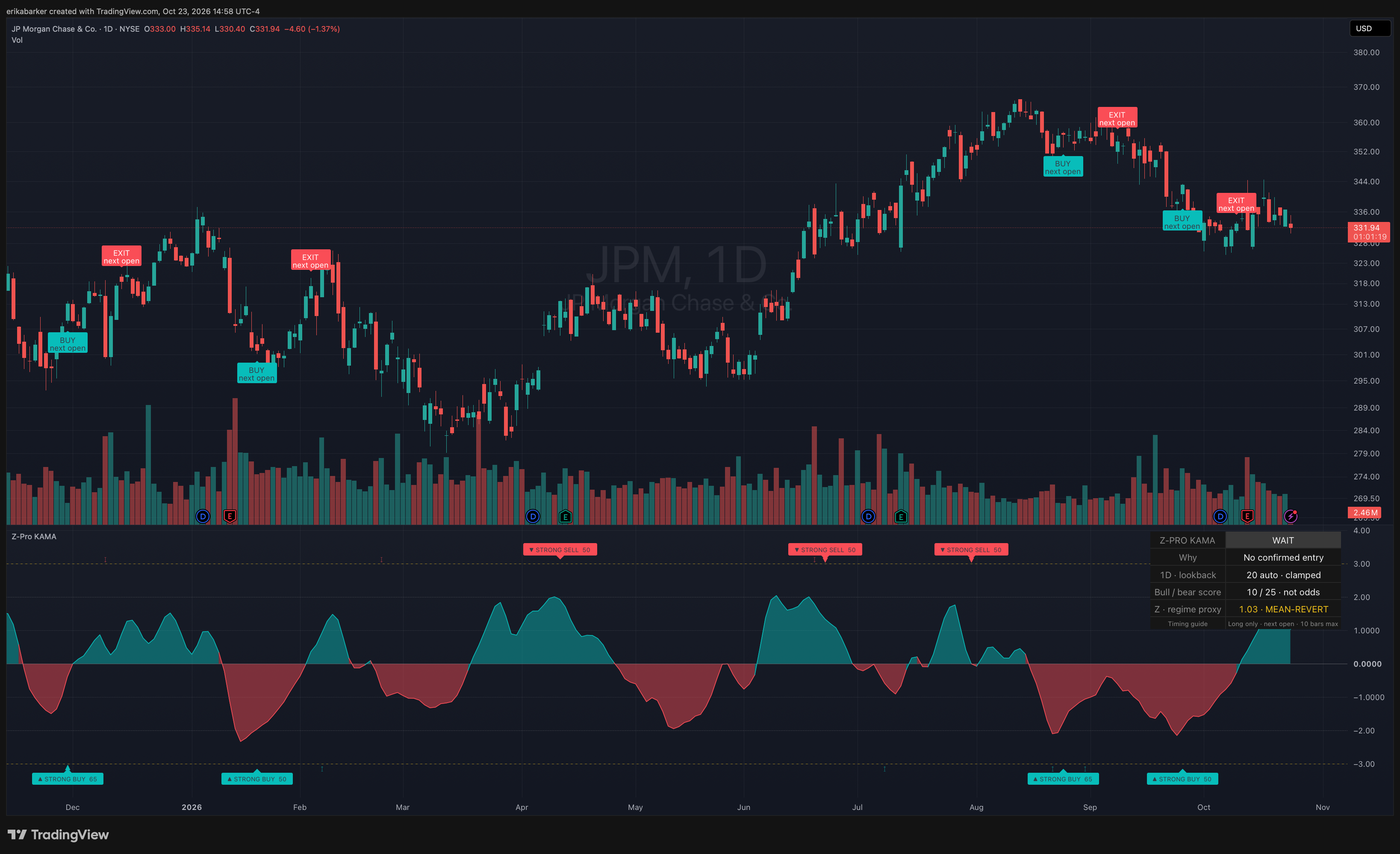
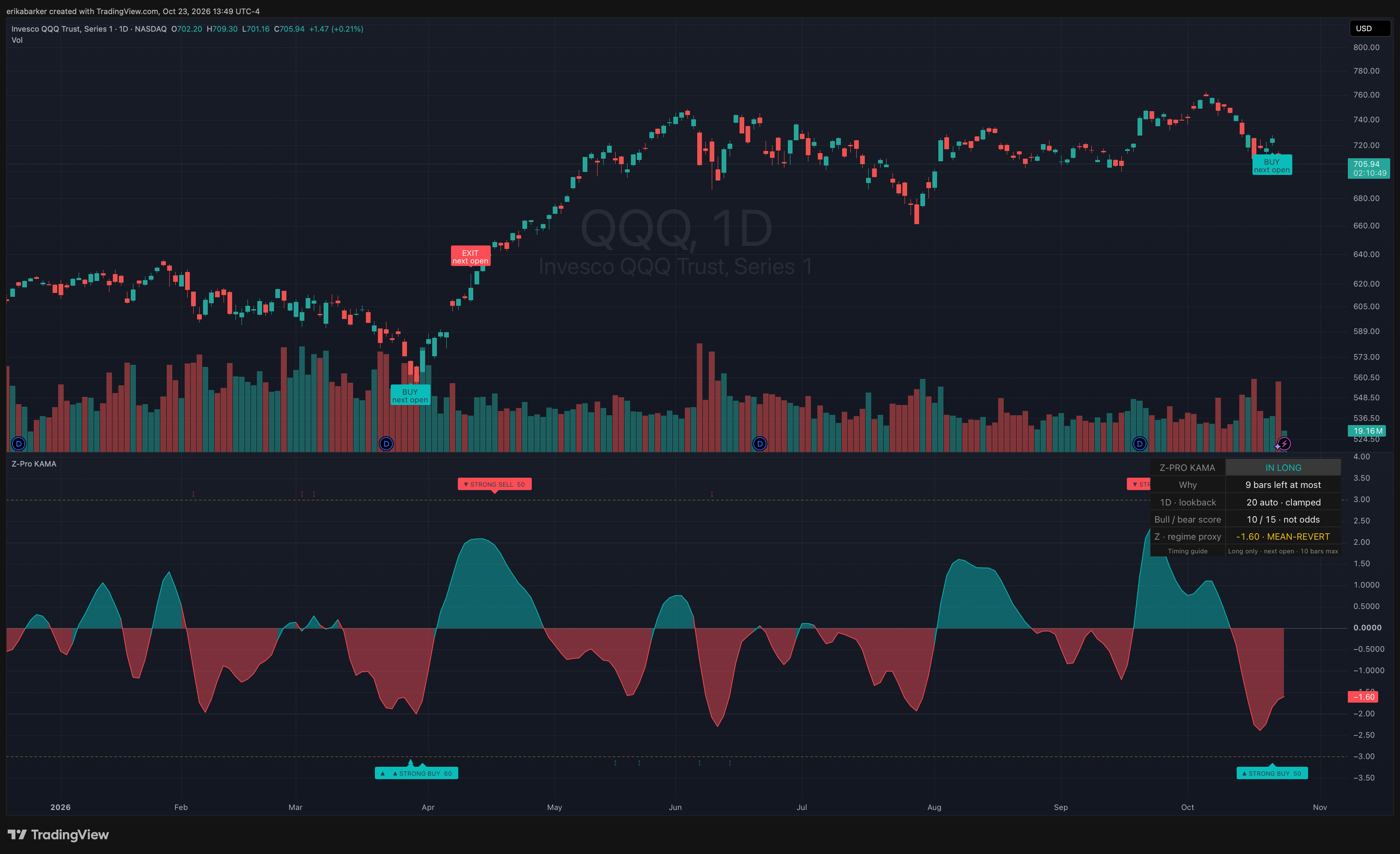
The script also includes a hypothetical long-only timing guide with BUY NEXT OPEN and EXIT NEXT OPEN labels. Its stated policy exits after an opposite qualifying signal or a ten-bar holding horizon. Those labels make one possible trading interpretation explicit. They do not know a reader’s holdings, objectives, or tax situation, and the indicator does not place orders.
The QQQ interface snapshot shows the oscillator, chart labels, and dashboard together. It illustrates how the tool presents information; the particular historical chart is not proof of an edge.
How I would approach it as a reader
For an individual trader, I would start with the question behind the reading. What moved? Relative to which baseline? Over what window? What changed in the company, sector, or broader market? Is this ordinary variation, or is there a reason the old reference may be less useful?
That does not require stacking six more indicators on the chart. More displays can make it harder to identify which observation actually changed your judgment.
If standard deviation is still unfamiliar, use the indicator as a way to learn before treating its labels as trading instructions. Plot the same market across several periods. Watch how the reference moves. Record what you expected before looking at what happened next. A student of markets or economics can use that exercise to study how descriptions, explanations, and predictions differ.
For an institutional research team, the open code offers a possible feature to investigate. Researchers could reproduce its calculations in their own system, compare it with simpler baselines, test whether it adds information beyond existing signals, and examine performance across regimes, costs, and capacity. Useful incremental information would have to earn its place.
That is the case I would make to a researcher at a firm such as Citadel or Jane Street. It is a possible research use, not a claim of adoption or endorsement. A sophisticated team may find something useful, modify it substantially, or conclude it adds nothing. Institutional experience does not make a weak signal strong, and thoughtful independent researchers can ask the same hard questions.
The original HMA indicator remains available, and so does the current KAMA version. The HMA listing records its original publication as August 27, 2024, with updates on April 14, 2025. I had developed the indicator before writing about it; the listing date is a separate milestone. Both tools belong to a project I am still learning from.
I still like the moment when a chart makes a complicated idea easier to see. I am simply more interested now in what happens after that moment: opening the code, checking the assumptions, and asking what would make me change my mind.